Cooling System for Hydrodynamic Bearing in Co2 Power CYcle
For a class this Fall 2025, I was the design and analysis lead for a class project to design the cooling system for a hydrodynamic bearing that holds the turbine of a CO2 power cycle. The cooling circuit was required to pull from one of the states in the power cycle, and be routed to the bearing, which has a constriction area of 6 mm^2. In the bearing, the heat generated will be from windage losses which is based on the density inside the bearing (which we were told to treat as constant after the constriction of the bearing area). Our system was to function in 8 different ambient states that the power cycle operates in ranging from -14°C to 85°C. The main specification of the project was that the CO2 leaving the bearing cannot be more than 100°C and that the flow inside the bearing could not undergo phase change.
Our design incorporates two valves, one before the bearing and one after the bearing. We pulled our CO2 from state 2 which we chose because of its low initial temperature and the high pressure that can drive flow across our system. We finished our circuit in state 6 because the pressure is lower, and additionally the mixing of fluids that will lower the temperature of state 6 can be adjusted for with the cooling water in the heat exchanger. Therefore our design would mitigate any major changes to the states which could lead to power loss. Through my analysis in google sheets—using a CoolProp template to gain access to the Propssi function—I found that the design would be best because the first valve can drop the pressure to a value above the critical pressure to ensure no phase change.
The second valve would control the pressure after the flow constriction—because we assumed isobaric heating through the bearing—and the pressure would then drop to the appropriate pressure of state 6. With our first valve we wanted to regulate the mass flow of our circuit to minimize turbine power losses, because the mass flow rate that we take out of the power cycle to use for our cooling means less mass flow over the turbine. These calculations are shown in Fig 5. and I found that the percent of power loss would be 2.5% at its highest. With the mass flow set at 0.1 kg/s, I focused on optimizing the valves by narrowing down their Cv ranges which helped us select our Badger Meter US Type 807 Small Control Valve in 1/2” size. The trims were slightly different for the two valves, but both had a high level of controllability for their short ranges of Cv values (theory of operations found in Fig 6.
If you are interested you can view the entire google sheet by going to this link
Calculations Sheet
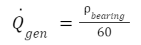
Fig 1. Heat generated equation from the windage losses, based on the density after the bearing constriction
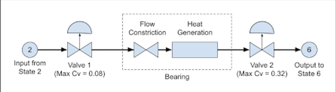
Fig 2. Overview of design pulling from state 2, flowing through one valve, through the constriction of the bearing and the bearing area, through one more valve and to state 6
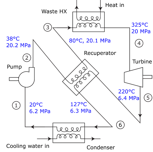
Fig 3. Power cycle that the CO2 was pulled from, for our design we pulled from state 2
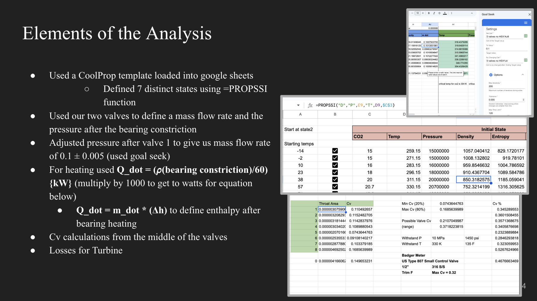
Fig4. Here is a slide of our design presentation that detailed how I analyzed the cooling circuit
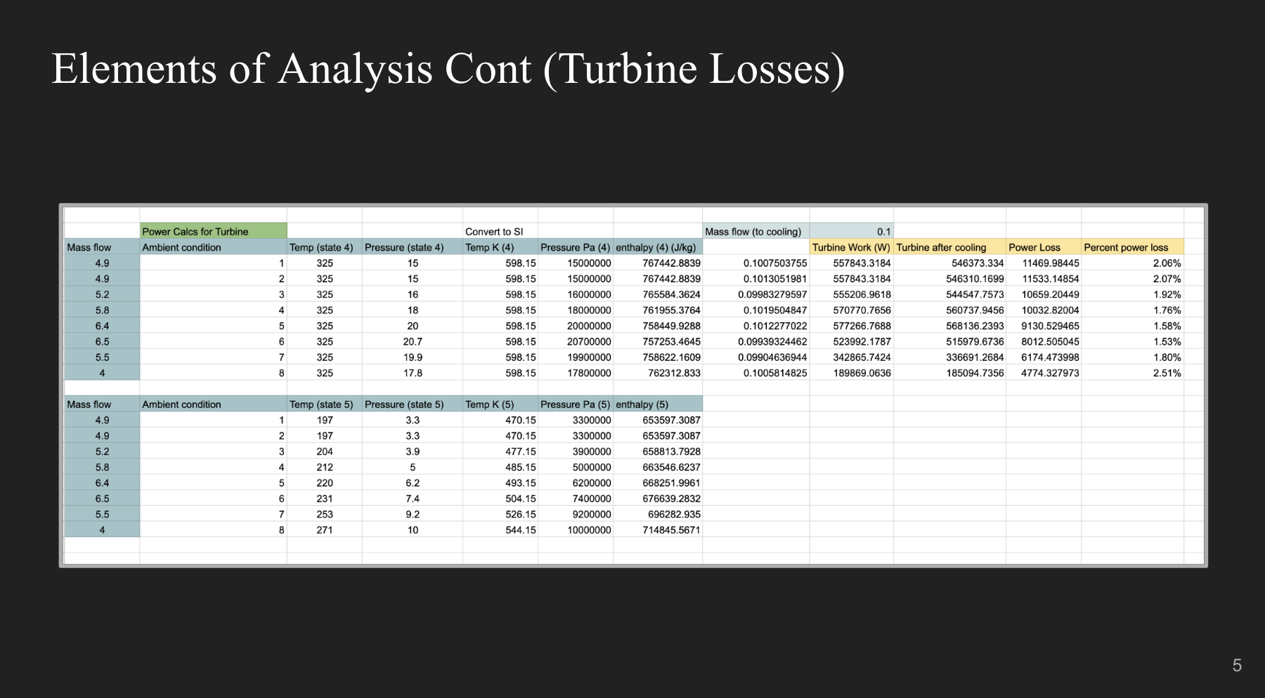
Fig 5. Follow up slide of analysis that showed how I calculated the percent loss that affects the overall power cycle, by finding the difference between the mass flow rate of the power cycle and the mass flow rate pulled into our cooling circuit.
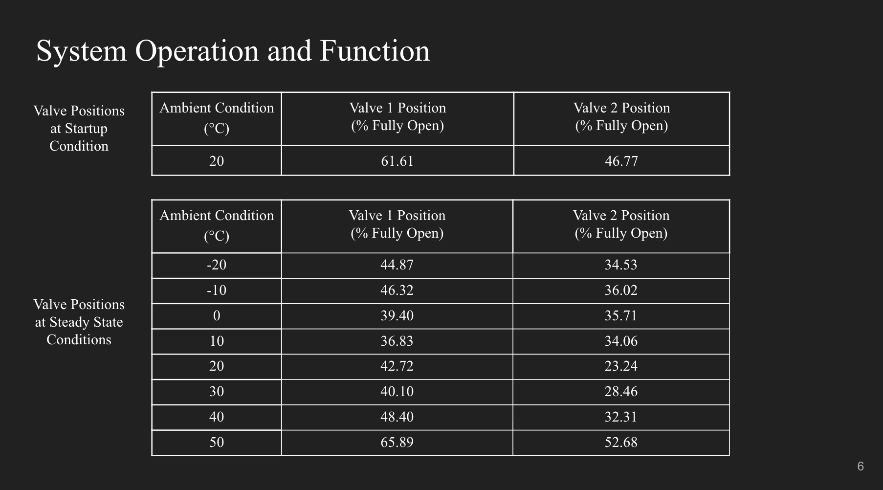
Fig 6. Theory of operations for our valves, showing how they will function at different ambient states.